
Debiased score test of the null fit.0 against the alternative
fit.1, both fitted with mgcv::gam. GLM fit.1 is
used to hunt for signal that fit.0 potentially misses.
Usage
# S3 method for class 'gam'
compare_models(
  fit.0,
  fit.1,
  hunt.style = "optimal",
  trim.outlier.hunt = TRUE,
  splits = c(0.5, 0.5),
  verbose = FALSE,
  ...
)
Arguments
- fit.0
The null model as a fitted
mgcv::gamobject.- fit.1
The alternative model as a fitted
mgcv::gamobject. Must be a supermodel offit.0: every predictor variable infit.0's formula must also appear infit.1's.fit.0andfit.1must be fit on the same rows in the same order.- hunt.style
Hunting algorithm with the following options.
'optimal': optimal hunting (default). Seehunt_optimal.'wls': a simpler hunting using weighted least squares, which can be less powerful. Seehunt_wls.
- trim.outlier.hunt
If
TRUE(default), extreme values produced by the hunted function will be trimmed using Tukey's IQR rule.- splits
Numeric vector of length 2 or 3 giving the relative sizes of the sample splits; rescaled internally to sum to one. Default is
c(0.5, 0.5), which splits data into two halves for hunt and test respectively. Though typically unnecessary in practice, one can also specify a 3-way split for hunt, debiasing and test respectively.- verbose
Default
FALSE; information is printed if set toTRUE.- ...
Unused; present for S3 generic/method consistency.
Value
An object of class "dScoreTest": a list whose key elements
are the debiased test statistic t.stat and the one-sided p-value
p.val (right tail of the standard normal), along with the test-set
score residuals, the hunted direction, and the call. It has
print,
summary and
plot methods.
Details
Nesting is checked by predictor-variable name only, not by basis span:
two models with the same predictors but different smooth specifications
(e.g. s(x, k = 5) vs s(x, k = 20)) will pass the check.
The test remains meaningful as long as fit.1's class contains the
relevant alternative directions. Factor predictors, offset() terms,
weights arguments, and multi-column responses are not supported.
Examples
set.seed(42)
dat <- mgcv::gamSim(eg=1, n=500, dist="normal", scale=1)
#> Gu & Wahba 4 term additive model
dat <- dat[, 1:5]
# test fit.0 against fit.1: well-specified (f3 = 0) and should not be rejected
fit.0 <- mgcv::gam(y ~ s(x0) + s(x1) + s(x2), data = dat)
fit.1 <- mgcv::gam(y ~ s(x0) + s(x1) + s(x2) + s(x3), data = dat)
compare_models(fit.0, fit.1)
#> Debiased score test:
#> y ~ X, with X consists of x0, x1, x2, x3.
#> (hunt.style = optimal, hunt.method = gam, debias.method = standard)
#> n = 500, two-way split: hunt = 250, debias & test = 250
#>
#> T = 0.2087, p-value = 0.417349
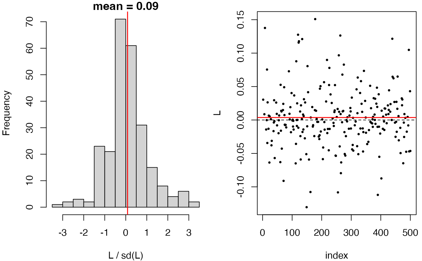
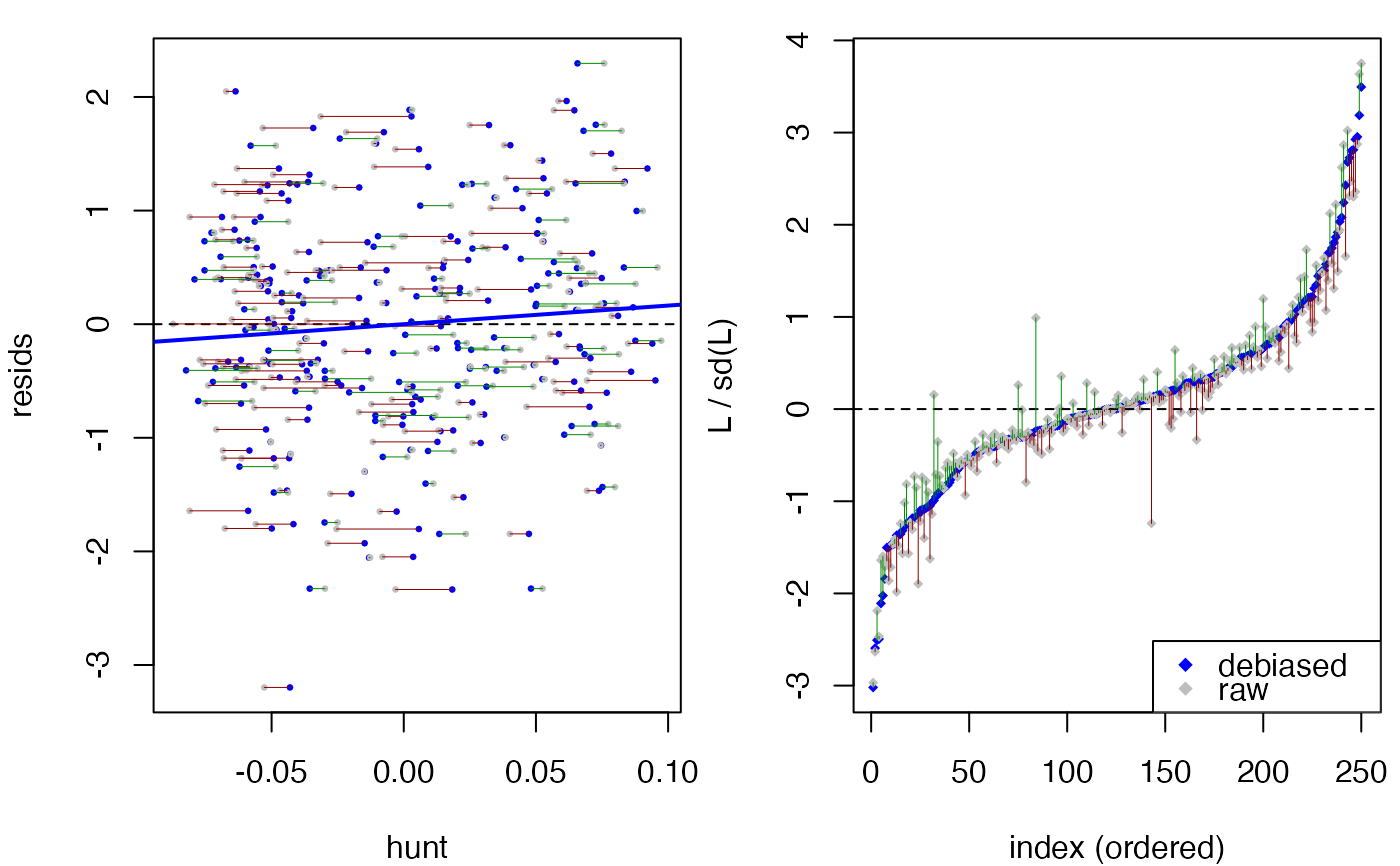
plot(compare_models(fit.0, fit.1))
 anova(fit.0, fit.1)
#> Analysis of Deviance Table
#>
#> Model 1: y ~ s(x0) + s(x1) + s(x2)
#> Model 2: y ~ s(x0) + s(x1) + s(x2) + s(x3)
#> Resid. Df Resid. Dev Df Deviance F Pr(>F)
#> 1 481.96 476.24
#> 2 476.00 466.58 5.9557 9.6527 1.6634 0.1287
# mis-specified model: drops f2 and should be rejected
fit.00 <- mgcv::gam(y ~ s(x0) + s(x1) + s(x3), data = dat)
compare_models(fit.00, fit.1)
#> Debiased score test:
#> y ~ X, with X consists of x0, x1, x2, x3.
#> (hunt.style = optimal, hunt.method = gam, debias.method = standard)
#> n = 500, two-way split: hunt = 250, debias & test = 250
#>
#> T = 13.7484, p-value = 2.60309e-43
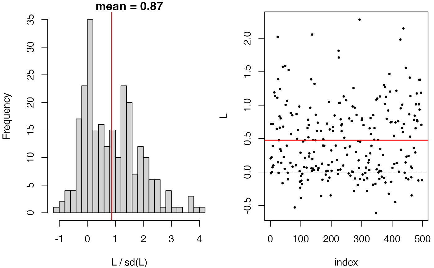
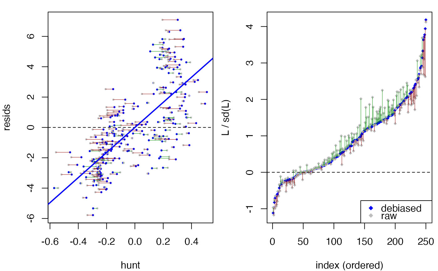
plot(compare_models(fit.00, fit.1))
anova(fit.0, fit.1)
#> Analysis of Deviance Table
#>
#> Model 1: y ~ s(x0) + s(x1) + s(x2)
#> Model 2: y ~ s(x0) + s(x1) + s(x2) + s(x3)
#> Resid. Df Resid. Dev Df Deviance F Pr(>F)
#> 1 481.96 476.24
#> 2 476.00 466.58 5.9557 9.6527 1.6634 0.1287
# mis-specified model: drops f2 and should be rejected
fit.00 <- mgcv::gam(y ~ s(x0) + s(x1) + s(x3), data = dat)
compare_models(fit.00, fit.1)
#> Debiased score test:
#> y ~ X, with X consists of x0, x1, x2, x3.
#> (hunt.style = optimal, hunt.method = gam, debias.method = standard)
#> n = 500, two-way split: hunt = 250, debias & test = 250
#>
#> T = 13.7484, p-value = 2.60309e-43
plot(compare_models(fit.00, fit.1))
 compare_models(fit.00, fit.1, hunt.style="wls")
#> Debiased score test:
#> y ~ X, with X consists of x0, x1, x2, x3.
#> (hunt.style = wls, hunt.method = gam, debias.method = standard)
#> n = 500, two-way split: hunt = 250, debias & test = 250
#>
#> T = 13.2812, p-value = 1.48754e-40
anova(fit.00, fit.1)
#> Analysis of Deviance Table
#>
#> Model 1: y ~ s(x0) + s(x1) + s(x3)
#> Model 2: y ~ s(x0) + s(x1) + s(x2) + s(x3)
#> Resid. Df Resid. Dev Df Deviance F Pr(>F)
#> 1 491.06 3974.4
#> 2 476.00 466.6 15.062 3507.8 239.02 < 2.2e-16 ***
#> ---
#> Signif. codes: 0 ‘***’ 0.001 ‘**’ 0.01 ‘*’ 0.05 ‘.’ 0.1 ‘ ’ 1
compare_models(fit.00, fit.1, hunt.style="wls")
#> Debiased score test:
#> y ~ X, with X consists of x0, x1, x2, x3.
#> (hunt.style = wls, hunt.method = gam, debias.method = standard)
#> n = 500, two-way split: hunt = 250, debias & test = 250
#>
#> T = 13.2812, p-value = 1.48754e-40
anova(fit.00, fit.1)
#> Analysis of Deviance Table
#>
#> Model 1: y ~ s(x0) + s(x1) + s(x3)
#> Model 2: y ~ s(x0) + s(x1) + s(x2) + s(x3)
#> Resid. Df Resid. Dev Df Deviance F Pr(>F)
#> 1 491.06 3974.4
#> 2 476.00 466.6 15.062 3507.8 239.02 < 2.2e-16 ***
#> ---
#> Signif. codes: 0 ‘***’ 0.001 ‘**’ 0.01 ‘*’ 0.05 ‘.’ 0.1 ‘ ’ 1