Checking generalized additive models • dScoreTest

library(dScoreTest)
library(mgcv)

This article walks through gof_test() and compare_models() on mgcv::gam fits. Because these examples lean on grf and refit GAMs across sample splits, they are slower than the package vignette — this is a web-only article (not run by R CMD check).

Simulation example

We simulate from the four-term additive truth in mgcv::gamSim(eg = 1), $y = f_0(x_0) + f_1(x_1) + f_2(x_2) + f_3(x_3) + \varepsilon,$ where $f_3 \equiv 0$ and $f_0, f_1, f_2$ are nonlinear. The covariates are independent uniforms.

set.seed(42)
dat <- gamSim(eg = 1, n = 400, dist = "normal", scale = 2, verbose = FALSE)

Goodness of fit

gof_test() checks the functional form of a fitted model against a nonparametric alternative built with a regression forest. A correctly specified additive smooth model is not rejected:

fit.smooth <- gam(y ~ s(x0) + s(x1) + s(x2) + s(x3), data = dat)
gof_test(fit.smooth)
#> Debiased score test: 
#> y ~ X, with X consists of x0, x1, x2, x3.
#> (hunt.style = optimal, hunt.method = grf)
#> n = 400, two-way split: hunt = 200, debias & test = 200
#> 
#> T = 0.6274, p-value = 0.265214

Formally, the above tests that the regression function $E[Y \mid X_0,X_1,X_2,X_3]$ is an additive function of $X_0,X_1,X_2,X_3$ . In contrast, if we specify that the regression function is a linear function of $X_0,X_1,X_2,X_3$ , the model is rejected.

fit.linear <- lm(y ~ x0 + x1 + x2 + x3, data = dat)
gof_test(fit.linear)
#> Debiased score test: 
#> y ~ X, with X consists of (Intercept), x0, x1, x2, x3.
#> (hunt.style = optimal, hunt.method = grf)
#> n = 400, two-way split: hunt = 200, debias & test = 200
#> 
#> T = 9.7238, p-value = 1.19302e-22

In fact, since $f_3=0$ in the data-generating mechanism, an additive regression model without s(x3) is still well-specified.

fit.drop3 <- gam(y ~ s(x0) + s(x1) + s(x2), data = dat)
gof_test(fit.drop3)   # f3 = 0, still well-specified given (x0, x1, x2)
#> Debiased score test: 
#> y ~ X, with X consists of x0, x1, x2.
#> (hunt.style = optimal, hunt.method = grf)
#> n = 400, two-way split: hunt = 200, debias & test = 200
#> 
#> T = -2.3486, p-value = 0.990578

Note: gof_test should not be used for testing significance of a predictor, as illustrated below.

fit.drop23 <- gam(y ~ s(x0) + s(x1), data=dat)
gof_test(fit.drop23)
#> Debiased score test: 
#> y ~ X, with X consists of x0, x1.
#> (hunt.style = optimal, hunt.method = grf)
#> n = 400, two-way split: hunt = 200, debias & test = 200
#> 
#> T = -0.4014, p-value = 0.655919

Since the model is only fitted on x0 and x1, the above tests $E[Y \mid X_0, X_1] = f_0(x_0) + f_1(x_1)$ as opposed to $E[Y \mid X_0, X_1, X_2, X_3] = f_0(x_0) + f_1(x_1),$ simply because gof_test does not see predictors x_1 and x_2 which do not appear in the model’s formula (you can see this from the printout y ~ X, with X consists of x0, x1). To ask whether one or more omitted covariates carries signal, use compare_models(), which gives the hunt access to the alternative’s covariates.

Model comparison

compare_models() tests a null model against a larger alternative model and detects signal living in the alternative’s extra terms. Similar to ANOVA, this can be used to test significance of one or more predictors. For example, we can test the significance of $f_2$ by fitting a model without s(x2) and comparing it against the full model.

fit.full <- gam(y ~ s(x0) + s(x1) + s(x2) + s(x3), data = dat)
res <- compare_models(fit.drop23, fit.full)
res
#> Debiased score test: 
#> y ~ X, with X consists of x0, x1, x2, x3.
#> (hunt.style = optimal, hunt.method = gam)
#> n = 400, two-way split: hunt = 200, debias & test = 200
#> 
#> T = 11.8263, p-value = 1.42765e-32

This p-value correctly measures the significance of predictors x2, x3.

Diagnostics

plot() on a dScoreTest object shows diagnostic panels. For a rejected test, the hunted direction h lines up with the residuals, so L = resids * h has a clearly non-zero mean. Indeed, we see a large positive slope in the ‘resids vs hunt’ plot below.

plot(res)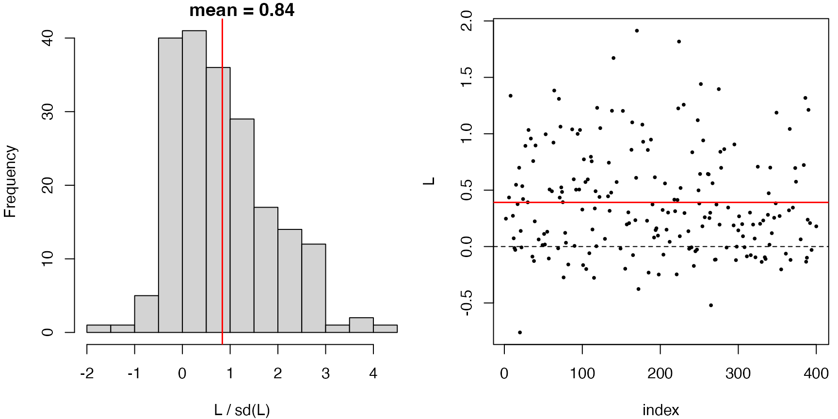

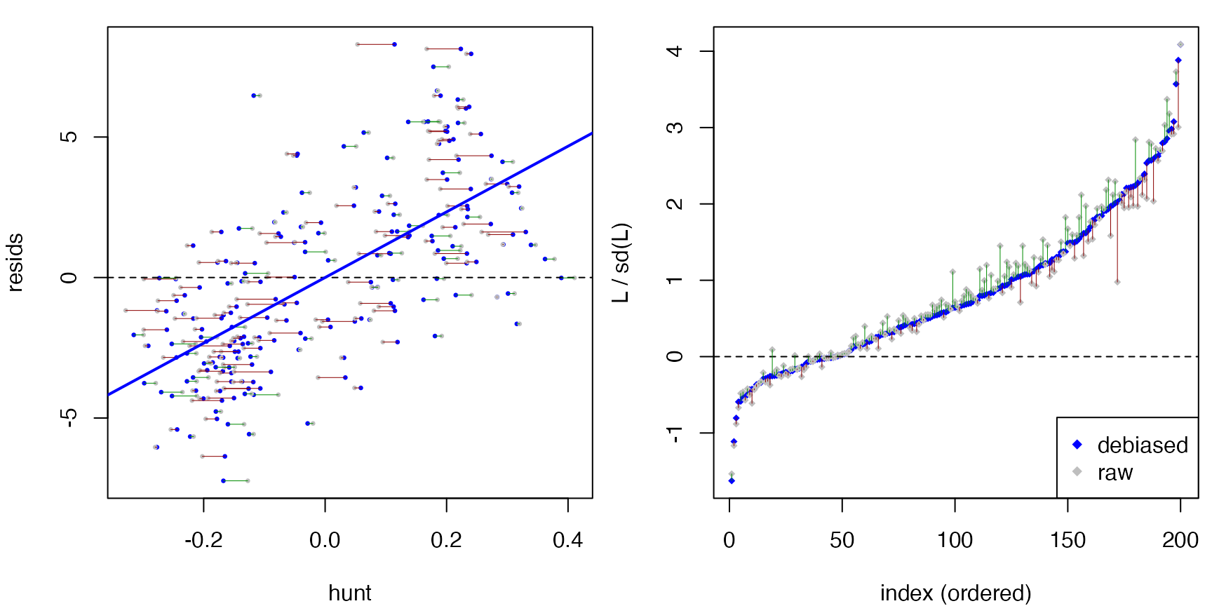
summary() adds a raw-vs-debiased comparison of the statistic, so you can see how much the outer orthogonalization step moved it:

summary(res)
#> Debiased score test
#> (hunt.style = optimal, hunt.method = gam)
#> n = 400, two-way split: hunt = 200, debias & test = 200
#> 
#>   Debiased:  T =  11.8263,  p = 1.42765e-32
#>   Raw:       T =  12.2269,  p = 1.11664e-34  (may contain bias)
#> 
#> L = resids * h (debiased):
#>     Min.  1st Qu.   Median     Mean  3rd Qu.     Max. 
#> -0.76145  0.01556  0.30110  0.39152  0.69664  1.91380 
#> 
#> L.raw = resids * h.raw:
#>     Min.  1st Qu.   Median     Mean  3rd Qu.     Max. 
#> -0.69498  0.02234  0.31879  0.39152  0.66576  1.85184 
#> 
#> h (debiased hunted direction):
#>     Min.  1st Qu.   Median     Mean  3rd Qu.     Max. 
#> -0.31512 -0.15726 -0.04016  0.00000  0.17892  0.38897 
#> 
#> h.raw (before outer debias):
#>      Min.   1st Qu.    Median      Mean   3rd Qu.      Max. 
#> -0.328412 -0.171114 -0.045389 -0.009752  0.174042  0.410749 
#> 
#> resids (score residuals on test):
#>    Min. 1st Qu.  Median    Mean 3rd Qu.    Max. 
#> -7.2341 -2.4313 -0.2759  0.0000  1.9564  8.2962

Hunt styles

All three hunts are available for GAMs. The optimal hunt is the default; the WLS hunt is simpler and sometimes nearly as powerful:

compare_models(fit.drop23, fit.full, hunt.style = "optimal")
#> Debiased score test: 
#> y ~ X, with X consists of x0, x1, x2, x3.
#> (hunt.style = optimal, hunt.method = gam)
#> n = 400, two-way split: hunt = 200, debias & test = 200
#> 
#> T = 10.0491, p-value = 4.63434e-24
compare_models(fit.drop23, fit.full, hunt.style = "wls")
#> Debiased score test: 
#> y ~ X, with X consists of x0, x1, x2, x3.
#> (hunt.style = wls, hunt.method = gam)
#> n = 400, two-way split: hunt = 200, debias & test = 200
#> 
#> T = 10.1919, p-value = 1.07797e-24

Example with prostate cancer data

In this section, we follow Wakefield (Bayesian and Frequentist Regression Methods, §12) to fit GAMs for analyzing the prostate cancer data in Stamey et al. (1989) and Tibshirani (1996).

prostate <- read.table(
  "https://hastie.su.domains/ElemStatLearn/datasets/prostate.data",
  header = TRUE)
prostate$train <- NULL
colnames(prostate)[c(1, 2, 4, 6, 9)] <-
  c("log.can.vol", "log.weight", "log.BPH", "log.cap.pen", "log.PSA")
head(prostate)
#>   log.can.vol log.weight age   log.BPH svi log.cap.pen gleason pgg45    log.PSA
#> 1  -0.5798185   2.769459  50 -1.386294   0   -1.386294       6     0 -0.4307829
#> 2  -0.9942523   3.319626  58 -1.386294   0   -1.386294       6     0 -0.1625189
#> 3  -0.5108256   2.691243  74 -1.386294   0   -1.386294       7    20 -0.1625189
#> 4  -1.2039728   3.282789  58 -1.386294   0   -1.386294       6     0 -0.1625189
#> 5   0.7514161   3.432373  62 -1.386294   0   -1.386294       6     0  0.3715636
#> 6  -1.0498221   3.228826  50 -1.386294   0   -1.386294       6     0  0.7654678

We want to use data to model the continuous outcome variable log.PSA, the log of prostate specific antigen (PSA), which is a biomarker to predict the clinical stage of cancer.

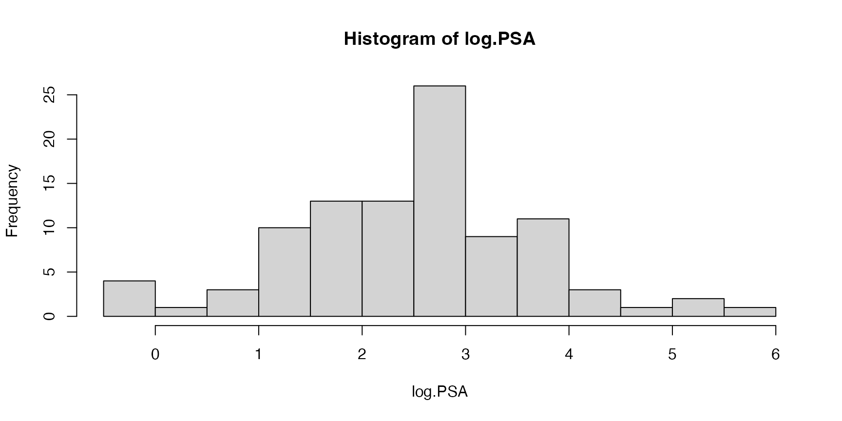
with(prostate, hist(log.PSA, breaks=15))

The dataset also measures the following covariates:

log.can.vol: log of cancer volume (cc), from the digitized tumor area times a thickness.
log.weight: log of the prostate weight (grams).
age: age of the patient (years).
log.BPH: log amount of benign prostatic hyperplasia, a noncancerous enlargement of the gland, as an area (cm²).
svi: seminal vesicle invasion, a 0/1 indicator of whether cancer cells have invaded the seminal vesicle.
log.cap.pen: log capsular penetration, the linear extent (cm) of cancer extending into the prostate capsule.
gleason: the Gleason score, a measure of tumor aggressiveness. Each of the two largest cancer areas is graded 1–5 (5 most aggressive) and the two grades are summed.
pgg45: the percentage of Gleason scores that are 4 or 5.

In particular, we want to model and visualize how log.PSA varies according to log.can.vol and log.weight, while accounting for other covariates. We fit a GAM model with penalized regression splines on each covariate, except for factors svi and gleason, which are introduced as simple linear terms. In particular, we fit two models for the joint effect of log cancer volume and log weight: one additive (no interaction) and one that adds a tensor-product interaction between them. Writing the bivariate part as ti() main effects plus a ti() interaction is the functional-ANOVA decomposition, so the interaction term captures only the interaction.

fit.0 <- gam(log.PSA ~ ti(log.can.vol, k = 6) + ti(log.weight, k = 6) +
                       s(age,         k = 7, bs = "cr") +
                       s(log.BPH,     k = 7, bs = "cr") +
                       s(log.cap.pen, k = 7, bs = "cr") +
                       s(pgg45,       k = 7, bs = "cr") +
                       svi + gleason,
             data = prostate, method = "GCV.Cp")

fit.1 <- gam(log.PSA ~ ti(log.can.vol, k = 6) + ti(log.weight, k = 6) +
                       ti(log.can.vol, log.weight, k = c(6, 6)) +   # interaction
                       s(age,         k = 7, bs = "cr") +
                       s(log.BPH,     k = 7, bs = "cr") +
                       s(log.cap.pen, k = 7, bs = "cr") +
                       s(pgg45,       k = 7, bs = "cr") +
                       svi + gleason,
             data = prostate, method = "GCV.Cp")

The two fitted surfaces are visualized as follows.

par(mfrow = c(1, 2))
vis.gam(fit.0, view = c("log.weight", "log.can.vol"), theta = 35, phi = 25,
        zlab = "fitted log.PSA", main = "without interaction")
vis.gam(fit.1, view = c("log.weight", "log.can.vol"), theta = 35, phi = 25,
        zlab = "fitted log.PSA", main = "with interaction")

Is the interaction model adequate?

Before testing the interaction, check that the model with interaction is itself well-specified:

set.seed(42)
gof.1 <- gof_test(fit.1)
gof.1
#> Debiased score test: 
#> y ~ X, with X consists of svi, gleason, log.can.vol, log.weight, age, log.BPH, log.cap.pen, pgg45.
#> (hunt.style = optimal, hunt.method = grf)
#> n = 97, two-way split: hunt = 48, debias & test = 49
#> 
#> T = -0.2882, p-value = 0.613421
plot(gof.1)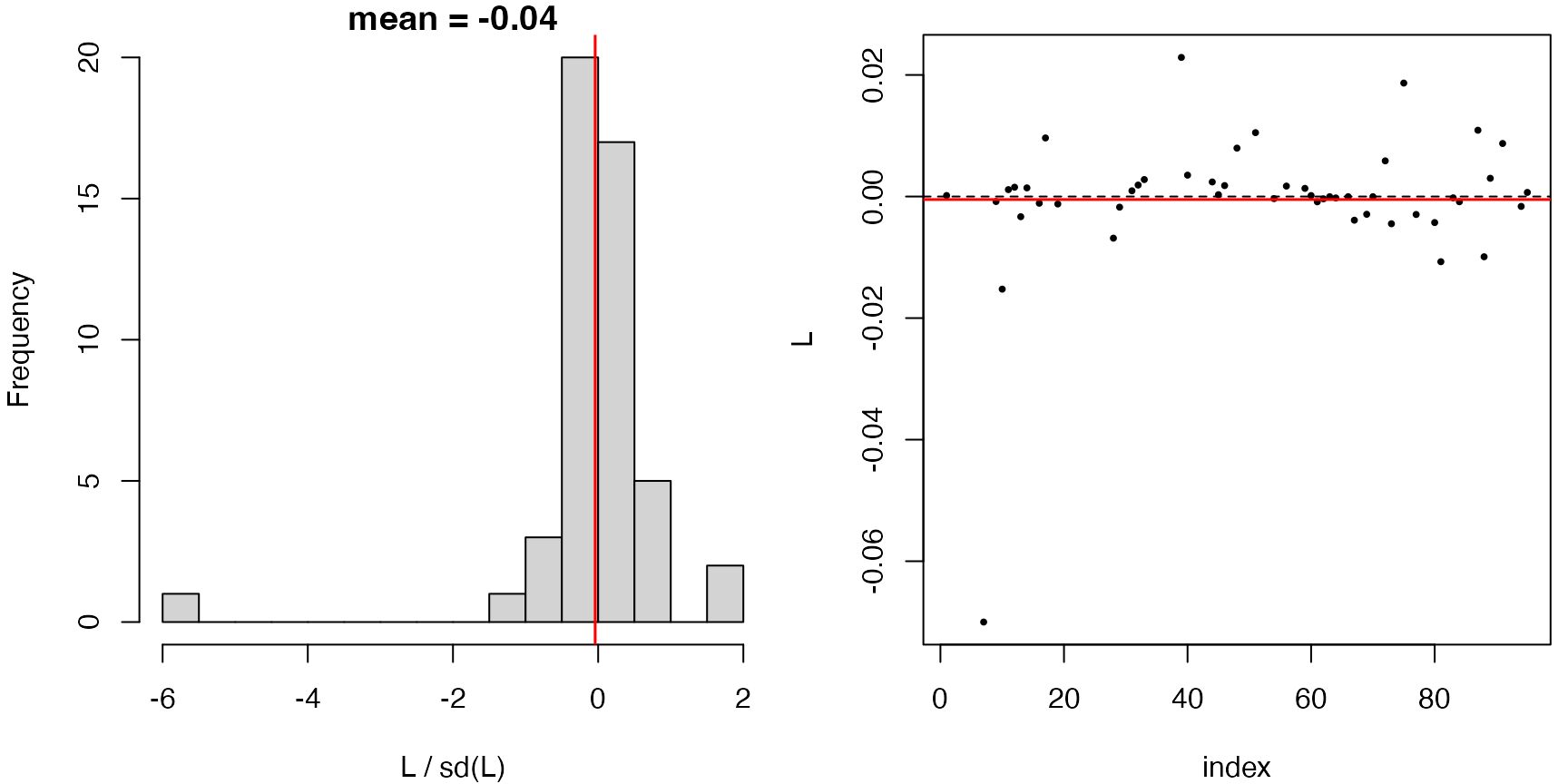

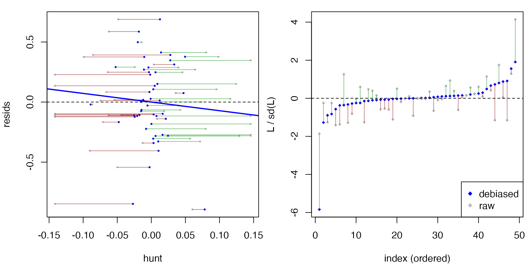
There is no indication of misspecification.

Testing for the interaction

compare_models() tests the additive null fit.0 against the interaction alternative fit.1:

set.seed(42)
compare_models(fit.0, fit.1)
#> Debiased score test: 
#> y ~ X, with X consists of svi, gleason, log.can.vol, log.weight, age, log.BPH, log.cap.pen, pgg45.
#> (hunt.style = optimal, hunt.method = gam)
#> n = 97, two-way split: hunt = 48, debias & test = 49
#> 
#> T = -1.5025, p-value = 0.933513

For comparison, mgcv’s own approximate significance test for the interaction term ti(log.can.vol,log.weight) is borderline significant.

summary(fit.1)$s.table
#>                                 edf   Ref.df         F      p-value
#> ti(log.can.vol)            1.703735 2.105484 15.045410 2.986785e-06
#> ti(log.weight)             1.000000 1.000000 11.902001 9.354714e-04
#> ti(log.can.vol,log.weight) 6.425780 8.669048  2.566460 1.553072e-02
#> s(age)                     3.408446 4.140520  2.469979 4.903984e-02
#> s(log.BPH)                 1.000000 1.000000  5.313203 2.400945e-02
#> s(log.cap.pen)             3.735876 4.332359  1.747032 1.315853e-01
#> s(pgg45)                   3.592971 4.312329  1.863861 9.226700e-02

Stabilizing across sample splits

With only 97 observations, a single debiased score test is sensitive to the random hunt/test split. Re-running it gives a spread of p-values:

set.seed(42)
replicate(10, compare_models(fit.0, fit.1)$p.val)
#>  [1] 0.93351306 0.06498306 0.52083874 0.28062263 0.95045012 0.95609299
#>  [7] 0.67061718 0.31334265 0.76105070 0.01090328

A practical remedy is to aggregate over many splits with a heavy-tailed combination test, which is robust to the strong dependence between splits (cf. the harmonic-mean p-value of Wilson, 2019):

set.seed(42)
pvals <- replicate(200, compare_models(fit.0, fit.1)$p.val)
1 / mean(1 / pvals)   # harmonic-mean p-value
#> [1] 0.01681002

The aggregated p-value seems to agree with the mgcv’s result.